Part 3 Animated graph

3.1 Data cleaning

I want to find out the studios that is above the lower quartile of average rating to see its rating change across 1958 to 2020. Thus, further data cleaning is needed.

summary(studiotop50$rating)

studiotop37r <- studiotop50 %>% 
  arrange(desc(rating)) %>% 
#after looking at the code, find out how many is below the 2.75 lower quartile
  slice (1:37)

#create a data set that contains only anime starting year, rating of the anime, and the name of the anime.
selectstudio <- anime1 %>% select(title, startYr, studios, rating)

selectstudioall <- merge(studiotop37r, selectstudio,by = "studios", all = TRUE)

#clean all the NA
selectstudioclean <- na.omit(selectstudioall)
#re name the heading
colnames(selectstudioclean) <- c("studios", "production","avg_rating","title","startyr","rating")

#create a list that is showing the studios average rating of each year.
newavg <- selectstudioclean %>% select(studios, rating, production, avg_rating,startyr)
newavg1 <- aggregate(newavg[, 2:4], list(newavg$studios, newavg$startyr), mean)
colnames(newavg1) <- c("studios","startyr","rating", "production","avg_rating")

3.2 Racing plot 1

This racing plot could show each year, which studio has highest average rating.

summary(selectstudioclean)

##    studios            production      avg_rating       title          
##  Length:4857        Min.   : 42.0   Min.   :2.756   Length:4857       
##  Class :character   1st Qu.: 99.0   1st Qu.:2.864   Class :character  
##  Mode  :character   Median :229.0   Median :3.196   Mode  :character  
##                     Mean   :265.9   Mean   :3.148                     
##                     3rd Qu.:339.0   3rd Qu.:3.276                     
##                     Max.   :683.0   Max.   :3.661                     
##     startyr         rating     
##  Min.   :1956   Min.   :0.000  
##  1st Qu.:1999   1st Qu.:2.732  
##  Median :2008   Median :3.322  
##  Mean   :2005   Mean   :3.166  
##  3rd Qu.:2014   3rd Qu.:3.852  
##  Max.   :2022   Max.   :4.702

library(gganimate)
library(av)
#create ranking list
newavg2 <- newavg1 %>% group_by(startyr)%>% 
  arrange(startyr, - rating)%>% 
  mutate(ranking = 1:n())

#Drop row that the year is above 2020.
newavg2 <-newavg2 [!(newavg2$startyr == "2021"|newavg2$startyr == "2022"),]

#Plot the graph
top1 <- ggplot(newavg2, aes(ranking, group = studios, 
                fill = as.factor(studios), color = as.factor(studios))) +
  geom_tile(aes(y = rating,
                height = rating,
                width = 0.9), alpha = 0.8, color = NA) +
  geom_text(aes(y = 0, label = paste(studios, " ")), vjust = 0.5, hjust = 0.5, size = 6, fontface="bold") +
  geom_text(aes(y=rating,label = round(rating, digits = 1)), colour = "black", hjust=1) +
  coord_flip(clip = "off", expand = FALSE) +
  scale_y_continuous(labels = scales::comma) +
#reverse display
  scale_x_reverse() +
  guides(color = FALSE, fill = FALSE) +
#set up theme i.e. the backgroud of the plot, the grid line etc
   theme(axis.line=element_blank(),
        axis.text.x=element_blank(),
        axis.text.y=element_blank(),
        axis.ticks=element_blank(),
        axis.title.x=element_blank(),
         axis.title.y=element_blank(),
        legend.position="none",
        panel.background=element_blank(),
        panel.border=element_blank(),
        panel.grid.major=element_blank(),
        panel.grid.minor=element_blank(),
        panel.grid.major.x = element_line( size=.1, color="grey" ),
        panel.grid.minor.x = element_line( size=.1, color="grey" ),
        plot.title=element_text(size=25, hjust=0.5, face="bold", colour="grey", vjust=1),
        plot.subtitle=element_text(size=17, hjust=0.5, face="italic", color="grey"),
        plot.caption =element_text(size=8, hjust=0.5, face="italic", color="grey"),
        plot.background=element_blank(),
       plot.margin = margin(2,2, 2, 4, "cm"),
       plot.tag.position = c (0.2, 0)) 

#animate the graph with label
anim = top1 + transition_states(startyr, transition_length = 4, state_length = 1) +
  view_follow(fixed_x = TRUE)  +
  labs(title = 'Studio average rating change by year : {closest_state}',  
       subtitle  =  "Top 37 Studio racing plot", tag = "Figure4: 1958-2020 Studio's raced rating change")

#nframes = 2 x length of the showing year (startyr). Without setting the plot will only show first 50 years
anime.gif <- animate(anim, nframes = 150, fps = 2.5, width = 1000, height = 1200)
anime.gif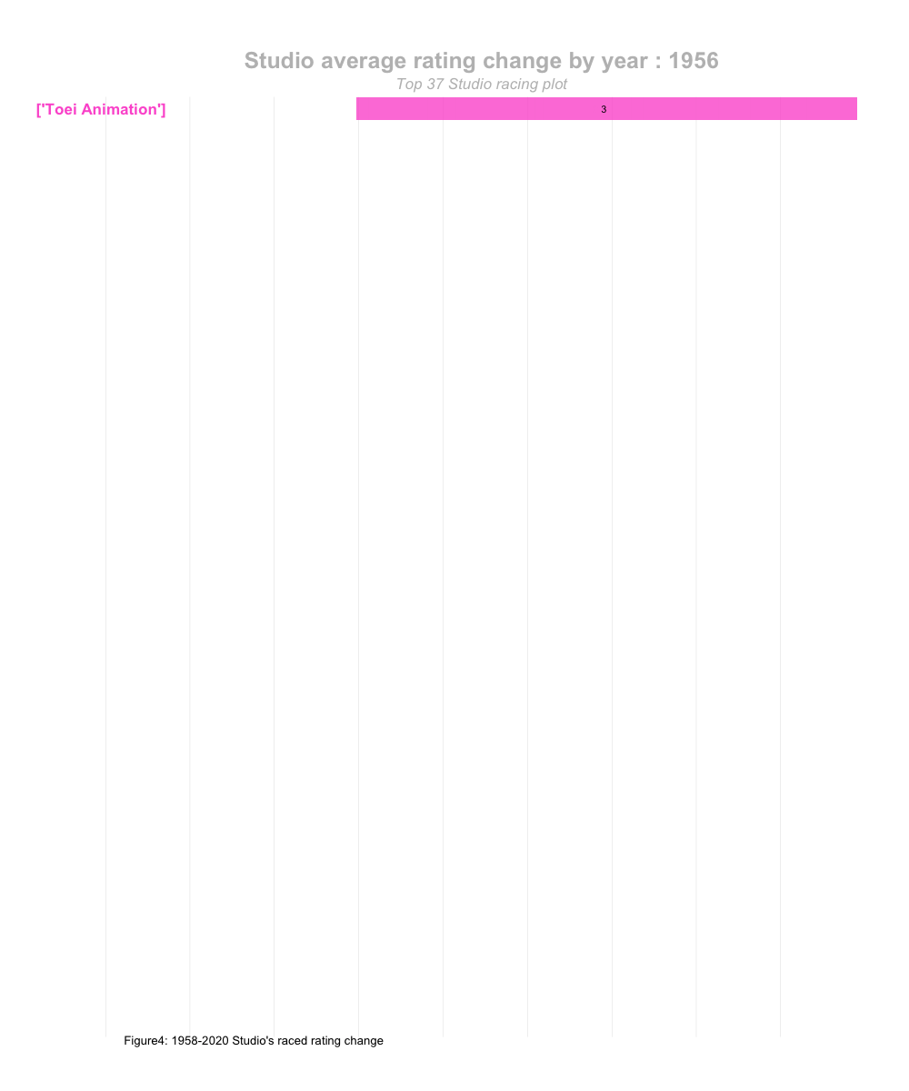

3.3 Racing plot 2

This plot fixing each studio’s position for better look or target a specific studio to visualise the rating change over the years.

topcompany <- ggplot(data=newavg2,aes (x = studios, y = rating, fill = rating))+
  geom_bar(stat = 'identity',size = 6, fontface="bold")+ 
  geom_text(aes(label=format(round(rating)), y=rating, hjust = -1),
            position=position_dodge(1)) + coord_flip()+
  #Let the colour change along with the rating
  scale_fill_gradient(low = 'grey39', high = 'cyan')+
  scale_y_continuous("rating") + theme_classic()+
  #Set up theme
  theme(legend.position='none', axis.text.y = element_text(size = 10, face = "bold"),
        plot.subtitle = element_text(size = 15, hjust = 1, vjust = -2, face = "bold"),
        plot.tag.position = c (0.3, 0))+
  #Animate the graph
  transition_states(states=startyr, transition_length=4, state_length = 1) +
  ease_aes('cubic-in-out') + labs (subtitle = 'Year:{closest_state}',
                                   tag = "Figure5: 1958-2020 Studio's rating change")+
  labs(x='Studio name')

anime1.gif <- animate (topcompany, nframes = 150, fps = 2, width = 600, height = 800)
anime1.gif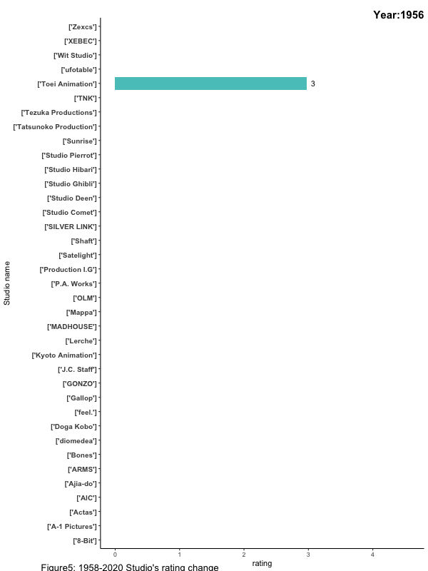

3.4 Racing plot on best studio

Merge data set first

#created a new dataset that merge top37 to the best studio
beststudior <- merge(newavg2, beststudio1, by = "studios", all = TRUE)
beststudior <- na.omit(beststudior)
beststudior <- beststudior%>% select(studios, startyr,rating.x,avg_rating,production.x,ranking)
colnames(beststudior) <- c("studios","startyr","rating","avg_rating", "production","ranking")

Plot the racing graph

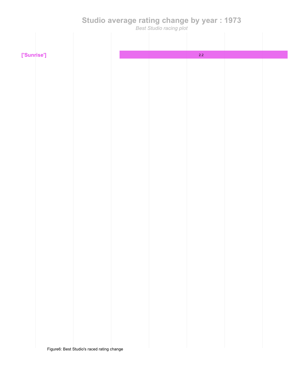
This plot shows the rate racing between the best studio each year.